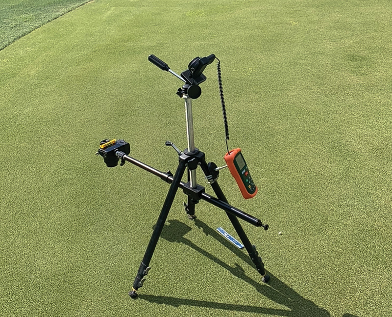
Figure 1. The camera setup used to take images of putting green turfgrasses in Florida in October 2020. The camera was positioned away from the tripod toward the sun to avoid interference from shadows. Also attached to the tripod was a light meter (orange) used to determine the intensity of incoming solar radiation at the time of image capture. The green in this image was Diamond zoysiagrass located in Orlando. Photo by W. Berndt
Color is an element of the health, quality and genetic expression of turfgrasses. It is also a characteristic used by turfgrass breeders to help make selections for the marketplace, and color may be a variable in turfgrass research events. Color response
to experimental treatments may be cited as a measure of treatment effectiveness or potential for turfgrass injury. Color may vary between turfgrass species and cultivars within species because of genetics, and it may be influenced by environmental
factors including the quality, intensity and duration of sunlight, soil type, and soil water content and quality. Anthropogenic factors that may influence turfgrass color include the level of applied nitrogen and the application of pigmented fungicides.
Biotic and abiotic stresses may also influence turfgrass color. The onset of drought stress or temperature stress or the application of pesticides and excessive traffic may change the color of swards.
Even though color is an important turfgrass characteristic contributing to its quality, and maintaining good turfgrass color is a major goal of most turfgrass management plans, golf course superintendents may not be familiar with the science behind assessing
turfgrass color. Lack of understanding of how color is scrutinized during research and breeding events may result in lesser understanding of what is reported in the turfgrass literature. The purpose of this article is to provide golf course superintendents
with information based on recently published research characterizing turfgrass colors using color spaces novel to the turfgrass literature. Having a better understanding of how turfgrass color can be assessed may help superintendents glean more knowledge
from the literature that shapes the evolution of turfgrass management.
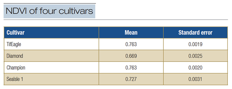
Table 1. Summary of the normalized difference vegetation index (NDVI) for 50 observations of four turfgrass cultivars cultured as putting greens in Florida in 2020.
Evaluating turfgrass color
There are differing ways to assess turfgrass color. The color of turfgrass may be characterized visually. Golf course superintendents may have either thought or said that their turf is off color, or they may have thought or said the turf “has great
color today.” Turfgrass researchers and breeders may characterize color using visual color ratings. Rating scores are typically between 1 and 9, with 9 being the most desirable color and 1 being least desirable. As with looking at turf and making
a visual judgment, this numerical assessment method is subjective and may be based largely on personal preferences for color and the level of experience one has in conducting the ratings.
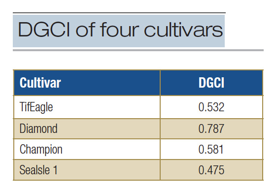
Table 2. Summary of the dark green color index (DGCI) as determined for four turfgrass cultivars cultured as putting greens in Florida in 2020.
Researchers may also use instrumentation to make objective color assessments. The instruments may include various colorimeters, optical sensors and spectral reflectance devices (5). Spectral reflectance is widely used in turfgrass science and in agriculture
and in certain applications produces what is known as the normalized difference vegetation index or NDVI. An NDVI score ranges from minus 1 to plus 1 and is considered a measure of greenness and plant density. High positive readings indicate a higher
level of plant greenness and density.
There are differing ways to obtain NDVI data using instruments ranging from hand-held devices to placing spectral reflectance devices on carts, drones or satellites. The NDVI scores obtained during research events are typically summarized using statistics
including analysis of variance or ANOVA. The ANOVA is used to determine if sets of NDVI scores differ. For example, Table 1 contains a summary of NDVI data obtained experimentally in Florida in 2020 for two hybrid bermudagrasses, TifEagle and Champion
[Cynodon dactylon (L.) Pers. var. dactylon x Cynodon transvaalensis Burtt-Davy]; a seashore paspalum, SeaIsle 1 [Paspalum vaginatum O. Swartz.]; and a zoysiagrass, Diamond [Zoysia matrella (L.) Merr.].
When subjected to ANOVA, it became apparent there were significant differences in NDVI scores between the cultivars (F=339, p<0.0001). In this case, the mean NDVI for Diamond zoysiagrass was significantly lower than for the bermudagrasses or the seashore
paspalum. These data might lead to the conclusion that the Diamond was not as green, or that the canopy was not as dense as the other cultivars. Or it could suggest that the Diamond has a different visible green color character.
Turfgrass color is also widely evaluated using digital photography paired with digital image analysis. As with spectral reflectance, digital imagery can be done with hand-held devices like digital cameras or by pairing digital cameras with drones or satellites.
One drawback with drones and satellites is the complexity of data acquisition and summation, and overall costs and expenses. It’s pretty tough to get time on a satellite, and if you do there is a steep learning curve. But hand-held digital cameras
are relatively inexpensive, and the methodology for taking digital images of turf to assess color is published in the literature.
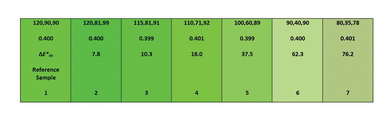
Figure 2. Each cell in the figure has a dark green color index value of 0.4 (second line of numbers) but differs visually compared to cell No. 1, which is a reference cell. All cells are green, and the given DGCI would infer that they’re all the same green color, but that’s not the case.
One variable associated with digital image analysis is called the dark green color index. The DGCI is a single measure of green color based on manipulation of the hue, saturation and brightness (HSB) color space (4). It’s like NDVI in that a single
number provides an estimate or measure of greenness. A color space or color model represents a way of organizing color components that is based on mathematics. Color spaces are usually 3D coordinate systems having various shapes, and there are different
kinds of color spaces that can be utilized to describe colors, but that is a topic in itself. With respect to the four cultivars in Table 1, the corresponding DGCI values as calculated for them are presented in Table 2.
These data may lead one to conclude that Diamond zoysiagrass has significantly more green color than the other cultivars. Dark green color index is a valuable tool for assessing turfgrass color, but readers should be aware that indices like DGCI and NDVI
can be misleading (Figure 2).
While indices like NDVI and DGCI are invaluable in helping to assess and communicate turfgrass color data to audiences, they are numbers, which may make it difficult for audiences to relate to the character of the color. This is because color is a visual sensation processed to be perceived. Perception refers to the way sensory information is organized, interpreted and consciously experienced. It’s difficult to perceive a color or perceive how colors may differ based solely on numbers or codes.
Matching turfgrass color(s) to published reference standards from the Munsell Plant Tissue Color Book (Munsell Color, Grand Rapids, Mich.) may help visualize and perceive color and assist in communicating color character to audiences. The way this works
is the user visually picks the published color chip from the Munsell book that most closely matches the color of the turfgrass. This is called visual color matching. The greatest benefit of this is that a visual link is established between the best-matching
Munsell color from the book and the turfgrass. Each color chip in the Munsell book is assigned a color code (e.g., 2.5G 8/4) that can be reported in writing. The color code represents the Munsell color space termed hue (base color), value (lightness
or brightness) and chroma (intensity) with the acronym H V/C. If a Munsell H V/C code is reported, then people can look up the code in the book and visualize (see) the color. The Munsell color system was created to assist in communicating and
evaluating colors and is considered a worldwide color standard for academia and industry.
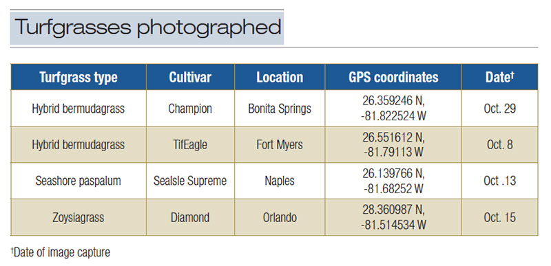
Table 3. Putting green turfgrasses photographed in Florida in October 2020.
Matching colors to published Munsell color chips is, however, a subjective visual comparison process, making it potentially prone to error. Error in color matching may occur because people may differ in ability to perceive colors, there may be distortion
due to lighting, and people may fail to adhere to color matching protocols. A more objective approach to matching turfgrass color to Munsell color standards could enhance the reporting of color data to audiences, making it more meaningful. Additionally,
it is difficult to link color indices like NDVI and DGCI, or other color variables or color spaces, directly to published Munsell colors.
In 2022, a novel method of assessing turfgrass digital colors based on digital image analysis was published in Crop Science (2). In addition, the authors developed a color matching algorithm for objectively assigning Munsell colors to turfgrasses. The
remainder of this current article is intended to provide an overview of how the digital color of turfgrass leaf blades was determined. Differentiating between the experimental colors (1) and objectively matching the experimental colors to published
Munsell color chips are to be addressed in a subsequent article.
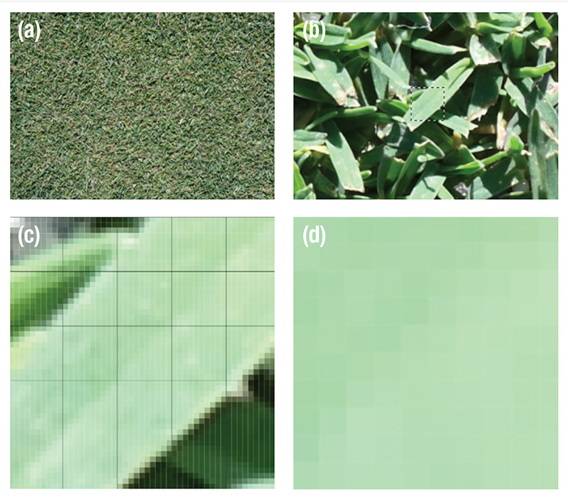
Figure 3. (a) Digital Image of putting green surface. The image size was 5,568 pixels by 3,712 pixels saved as 15-bit-plus L*a*b* mode with Photoshop. (b) Zoom, then examine each digital image visually to identify suitable individual leaf blades for image analysis. A portion of the leaf blade was selected using Photoshop (i.e., the dashed square). The selection was 50 pixels by 50 pixels, or 2,500 pixels. (c) Zoom to the 2,500-pixel selection of the individual leaf blade and install a virtual grid over the image using Photoshop. The grid consisted of 25 cells, each 10 pixels by 10 pixels, or 100 pixels. Five of the 100-pixel squares were selected and saved as independent images. The darkened square in the center of the image was one selection. (d) A 100-pixel L*a*b* color space sub-image of a leaf section within the leaf margins. This image was the square from the previous image. Commercial software was then used to determine the color of each of the 100 pixels in this sub-image. For each leaf blade, there were five sub-images within leaf margins, so that 500 pixels were measured per leaf blade, with 60 leaf blades per cultivar.
Digital images of leaf blades
Digital images of putting green turf were taken at each of three points on each of four putting greens referenced earlier (Figure 1, Table 3).
The digital images were taken using a Nikon Z50 20.9-megapixel (px) camera with a Nikkor Z-DX 16-50 mm lens (Nikon Corporation, Chiyoda, Japan). The camera was stabilized with a tripod, with the focal plane horizontal to, perpendicular to, and 10.6-11.8
inches (27-30 centimeters) from the turf surface. The initial images that were taken are what are called 16-bit raw images or NEF images (NEF is proprietary Nikon raw image format). There are 28 (256) possible colors in 8-bit images (like iPhone images),
while in 16-bit images there are 2.814 (1.8 million) possible colors, allowing for greater degrees of color discrimination. Ultimately, all images of turfgrass leaf blades were saved for image analysis as what are called 15-bit-plus CIE L*a*b* images
using Adobe Photoshop (Adobe Systems Inc., San Jose, Calif.). The L*a*b* as referenced is a 3D color space and is considered an opponent color model, where L* references perceptual lightness or brightness, the a* references green/red (magenta) opponent
colors, and the b* references blue/yellow opponent colors. The CIE L*a*b* color space is a Euclidian coordinate system that has been used for mapping colors visible to humans. In the current research, 100-pixel sections of individual turfgrass leaves
within leaf margins were examined for color composition (Figure 3).
Commercial software called PatchTool (The Babel Company, Montreal) was used to extract color space data from each pixel of the 100-pixel leaf sections. The color data was extracted in the form of the CIE L*a*b* color space as well as in a color space
termed CIE xyY color space (Figure 4).
The xyY color space is a chromaticity-luminance coordinate color space that is a normalized representation of perceived colors. One of the reasons that the xyY color space was used was that the xy portion of the xyY data can be plotted in two dimensions
on what is called the 1931 CIE 2-degree chromaticity diagram, which gives a basic indication of the colors (Figure 5).
When the 2D xy data for each of the cultivars were compiled and plotted on the chromaticity diagram, the data were then analyzed by performing a statistic called a cluster analysis. A cluster analysis is essentially describing whether there is a grouping
of data points sharing similar characteristics. As the data for this research was xy coordinate data, the cluster analysis examined the distances the xy points for each of the leaves were from each other.
And when the collective xyY data was plotted in 3D, the result was Figure 6.
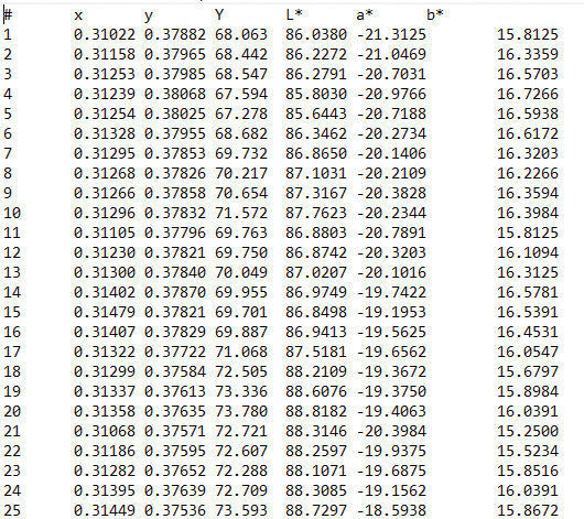
Figure 4. The first 25 color datapoints for a 100-pixel section of a turfgrass leaf blade from Figure 3. Both L*a*b* and xyY color space data were extracted from each leaf section using proprietary software. The cultivar associated with this data was Champion. There were 500 pixels per leaf blade, with 60 leaf blades per cultivar assessed during this research. Thus, for each cultivar, 30,000 pixels were evaluated for color character.
From the data plotted in Figure 6, it was apparent that data points for each cultivar were differentiated by a unique centroid describing its relative xy position. For Champion, 80% of xy data points were associated with centroid 4, while for TifEagle,
73% were associated with centroid 3. For Diamond, 92% of points were associated with centroid 2. SeaIsle Supreme had more disparity in xy, spanning four hue groups and was not assigned to any specific centroid. Compared to Champion, the Diamond was
darker with less lightness or brightness, thus appearing as a darker green color (Figure 7).
The mean Y (brightness or lightness) for Diamond was about 44, compared to about 61 for both TifEagle and Champion. Close examination of Figure 6 shows that each cultivar displayed a continuum of hues and lightness values; some leaves of Diamond appeared
to be the same color as those of both Champion and TifEagle. But generally, the color of Diamond did not appear to be the same as that of either TifEagle or Champion. It cannot be said that there were statistical color differences, because the images
were taken at differing locations on differing dates, but this research revealed that perceived colors of these cultivars were not the same.
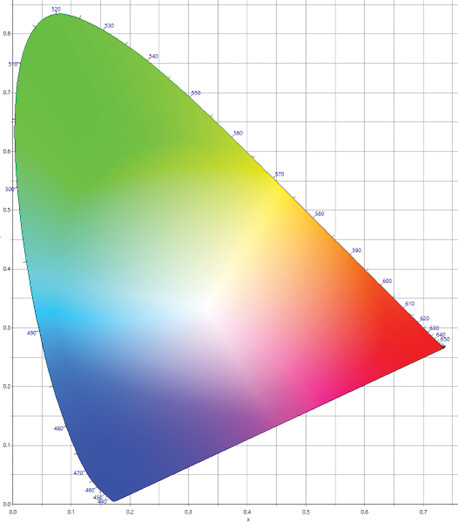
Figure 5. The 1931 CIE 2-degree chromaticity diagram. This figure is a graphical representation of the gamut of colors visible to humans based on the primary colors red, green, and blue. The horseshoe-shaped boundary is called the spectral locus. Wavelengths of light corresponding to colors are marked along the spectral locus. As xy coordinates appear closer to the spectral locus, the colors become more saturated or have a greater purity. Colors near the point where the colors converge are said to be more washed out. The point where the colors converge is called the white point where there is no color other than white.
Summary and Conclusions
Using the L*a*b* and xyY color spaces to describe the color of turfgrass leaves was part of a novel method of assessing color for turfgrass science. It’s the first time that the xyY color space has been used in turfgrass science to assess leaf colors.
The turfgrass literature generally references color indices such as NDVI or DGCI, while some turfgrass literature uses other color metrics, including hue angle, to help describe color (6). Introducing the L*a*b* and xyY color spaces to the turfgrass
community to help assess color introduces a more in-depth foray into the arena of color science, especially when coupled with analysis of 15-bit-plus resolution images.
Another novel aspect to this research is the focus on the color of individual leaves as opposed to turf per se. A benefit to doing this is that when a composite turf is analyzed, then the void spaces and shadows are also included in the analysis producing
color noise (Figure 8).
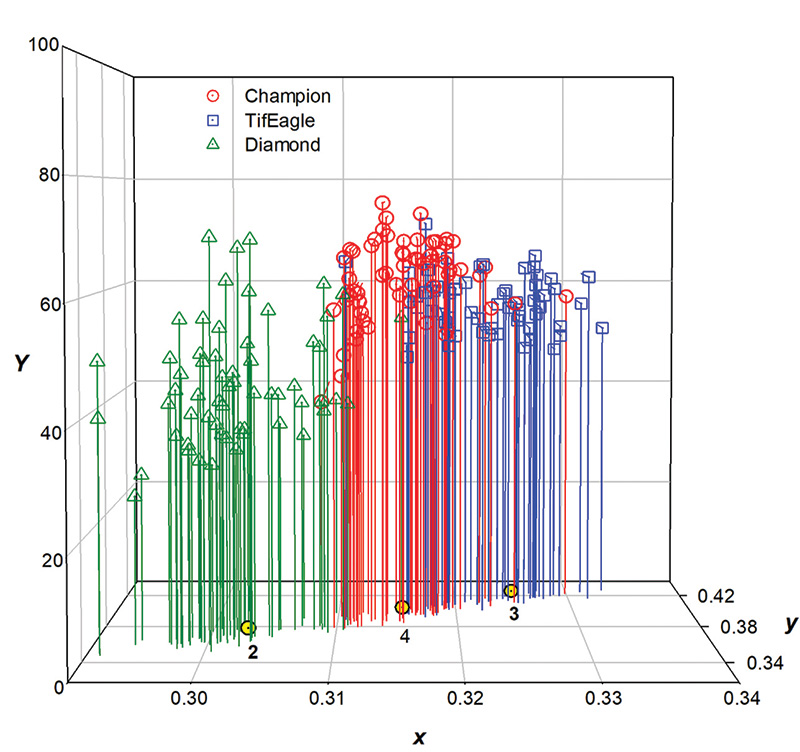
Figure 6. Plots of the xyY color of each of 60 individual leaf blades of three warm-season turfgrass cultivars. In this figure the vertical axis (Y ) refers to brightness or lightness. The xy plane gives hue or color as positioned in the CIE 1931 2-degree chromaticity diagram. The yellow dots on the xy plane represent separate and distinct clusters of data points called centroids.
When individual leaves are examined, a much cleaner view of cultivar color is produced (Figure 3); in turf images, dark or black pixels are present in void spaces or shadows. While it could be argued that an observer visually perceives all the colors
of a turf collectively (i.e., black, browns, yellows, etc.), it could also be argued that reflection of green from the leaf canopy is what the observer may really be focused on. This may give better representation of the true color of a cultivar or
species, at least as far as leaves are concerned. Thus, in procedures using DIA for turfgrasses, specifying turf color versus leaf color or the color of other plant parts would be prudent.
Another benefit to assessing color using the method as described involves costs. The Nikon digital camera that was used was under $1,000. A subscription to Adobe Photoshop is $10 per month, and the proprietary software used to extract color information
was about $125 for a lifetime license.
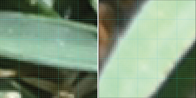
Figure 7. Visual comparison of digital images of leaf blades of Diamond zoysiagrass (left) and Champion hybrid bermudagrass (right) illuminated by full, unobstructed sunlight.
This procedure as outlined may not currently be suitable for use by superintendents in the field, as the workflow is somewhat tedious. However, the process using the L*a*b* and xyY color spaces could eventually be linked to smartphone technology, and
that is currently being worked on. Smartphone technology has already been used to establish L*a*b* color for soil images (3). Conversion of L*a*b* color space to xyY color space is relatively simple to do, and there are color space conversion calculators
online. Superintendents may also be able to take advantage of existing smartphone technologies. Commercial smartphone apps can interface with portable spectral reflectance devices to measure color (Measure Color Mobile; measurecolormobile.com), and
smartphone apps like ColorMeter RGB Colorimeter (White Marten GmbH, Baden-Wurttemberg, Germany) are available in the App Store (Apple, Cupertino, Calif.) for iOS systems. ColorMeter RGB Colorimeter provides color space metrics including L*a*b* from
smartphone images of surface reflectance colors.
The use of xyY color space as described in the current research is necessary to be able to match experimental colors to Munsell color chips as outlined (2). The color matching protocol is based on regression analysis and will be described in a follow-up
article. That article will also introduce superintendents to a method of differentiating colors by using L*a*b* color space parameters (1). In the meantime, superintendents may want to look at their turf and ask themselves, “What color is that?”
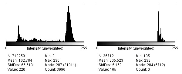
Figure 8. Histogram analysis of Champion turf (left) including pixels representing all visible colors associated with void spaces and shadows and other interfering color features versus a histogram of an individual Champion leaf blade within leaf margins (right). In this histogram (right), all the extracted color space coordinates are solely from the leaf blade, giving a more uniform appearance of green color, and possibly a more accurate representation of true cultivar color. Notice how clean the peaks are compared to the histogram on the left, which has considerable noise (i.e., lots of little peaks). The histograms look at all available pixels in an image, including black pixels, which contribute to void spaces.
The Research Says
- Color indices like NDVI and DGCI are valuable tools for assessing turfgrass color but may not provide an adequate summary of true color character.
- Assessing a pixel-by-pixel summary of color character can be done accurately and objectively using 15-bit-plus L*a*b* digital images saved in Adobe Photoshop and other proprietary imaging software.
- The research described in this article represents the first known use of xyY color space in turfgrass science.
- Utilizing novel concepts in turfgrass science shapes the evolution of turfgrass management.
Literature cited
- Berndt, W.L., D.E. Karcher and M.D. Richardson. 2020. Color-distance modeling improves differentiation of colors in digital images of hybrid bermudagrass. Crop Science 60(4):2138-2148 (https://doi.org/10.1002/csc2.20158).
- Berndt, W.L., and R.E. Gaussoin. 2022. Predicting Munsell color for turfgrass leaves. Crop Science (https://doi.org/10.1002/csc2.20843).
- Fan, Z., J.E. Herrick, R. Saltzman, et al. 2017. Measurement of soil color: A comparison between smartphone camera and the Munsell color charts. Soil Science Society of America Journal 81(5):1139-1146 (https://doi.org/10.2136/sssaj2017.01.0009).
- Karcher, D.E., and M.D. Richardson. 2003. Quantifying turfgrass color using digital image analysis. Crop Science 43(3):943-951 (https://doi.org/10.2135/cropsci2003.9430).
- Landschoot, P.J., and C.F. Mancino. 2000. A comparison of visual vs. instrumental measurement of color differences in bentgrass turf. HortScience 35(5):914-916 (https://journals.ashs.org/hortsci/view/journals/hortsci/35/5/article-p914.xml).
- Zhang, C., G.D. Pinnix, Z. Zhang, G.L. Miller and T.W. Rufty. 2017. Evaluation of key methodology for digital image analysis of turfgrass color using open-source software. Crop Science 57(2):550-558 (https://acsess.onlinelibrary.wiley.com/doi/abs/10.2135/cropsci2016.04.0285).
William L. Berndt (Leeberndt@aol.com, @Dr_Lee_Berndt) is a consulting agronomist specializing in golf course turfgrass management. He has a doctorate in botany and plant pathology from Michigan State University and is the author of numerous turfgrass
publications. A former college professor, he consults on golf courses, conducts research and performs expert witness work.